2. kNN for (Q)SPR modeling ⚛️

Goals of this exercise 🌟

• We will learn how to construct a simple SPR model using kNN

• We will learn the importance of data normalization (scaling)

• We will review the concepts of training and test split and cross-validation

• We will review some of the performance metrics for assesing classification models

A quick reminder ✅

Probably the simplest data-driven model that you can think of is k-nearest neighbours (kNN). It simply predicts future data as the average (or mode) of the “k” nearest neighbours of the queried point.

As simple as this idea might be, it works relatively good in various applications. One of them is the generation of (quantitative) structure-property relationships ((Q)SPR) models [SXG+03, YJQ+19]. Whether the word “Quantitative” is sometimes included or not depends on whether the model in question is a regression model or a classification model. Do you remember the difference?

The key question in kNN is what do we consider a neighbour and what not? This indicates us that we need to define a sort of similarity or distance metric that allows us to distinguish neighbouring points from points that are far away.

Common distance metrics use the different mathematical norms. For example, the Euclidean distance:

\[ d(\textbf{x}, \textbf{x'}) = \sqrt{\sum_i^D (x_i - x'_i)^2} \]

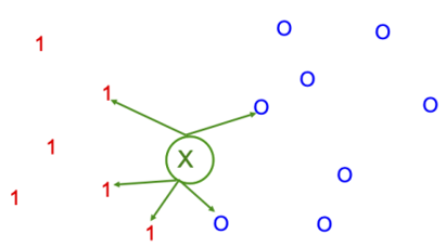
Fig. 5 Among the k-nearest neighbours (k=5), the majority of points are red 1s. Therefore, the queried point (green x) will be labeled as “red 1”. Image taken from [Mur22].

Let’s exemplify the use of kNN by constructing a SPR model that predicts the whether a molecule is mutagenic or not.

Mutagenicity is the property of substances to induce genetic mutation. It is one of the most important environmental, health and safety (EHS) properties to check when dealing with novel chemicals (e.g., drugs or solvents). In this case, we are going to use the data of mutagenicity on Salmonella typhimurium (Ames test). This dataset was collected by the Istituto di Ricerche Farmacologiche Mario Negri, merging experimental data from a benchmark dataset compiled by [HMS+09] from a collection of data made available by the Japan Health Ministry within their Ames (Q)SAR project.

Let’s fist import some libraries

import pandas as pd
import matplotlib.pyplot as plt
import seaborn as sn
import numpy as np
%matplotlib inline

Get data 📚

We have previously computed some molecular descriptors that will serve as input to our model. However, this is also an important step to consider when facing a problem like this: what are the important inputs to model mutagenicity? how do we know if these pre-computed features are enough for modeling mutagenicity? can we generate relevant molecular features automatically? 🤔

Ok, let’s use pandas to import the data as a DataFrame…

if 'google.colab' in str(get_ipython()):
  df = pd.read_csv("https://raw.githubusercontent.com/edgarsmdn/MLCE_book/main/references/mutagenicity_kNN.csv")
else:
  df = pd.read_csv("references/mutagenicity_kNN.csv")

df

	Unnamed: 0	Id	CAS	SMILES	Status	Experimental value	Predicted value	NumValenceElectrons	qed	TPSA	MolMR	BalabanJ	BertzCT	MolWt	MolLogP
0	0	1	100-00-5	O=[N+]([O-])c1ccc(cc1)Cl	Training	1	1	52	0.463602	43.14	38.1064	3.003401	244.429658	157.556	2.24820
1	1	2	100-01-6	O=[N+]([O-])c1ccc(N)cc1	Training	1	1	52	0.359544	69.16	37.5088	3.003401	242.429658	138.126	1.17700
2	2	3	100-02-7	O=[N+]([O-])c1ccc(O)cc1	Training	0	1	52	0.470728	63.37	34.7612	3.003401	241.674771	139.110	1.30040
3	3	4	100-11-8	O=[N+]([O-])c1ccc(cc1)CBr	Training	1	0	58	0.432586	43.14	45.7274	2.913802	257.648013	216.034	2.48970
4	4	5	100-12-9	O=[N+]([O-])c1ccc(cc1)CC	Training	0	0	58	0.479785	43.14	42.4744	2.913802	253.299498	151.165	2.15720
...	...	...	...	...	...	...	...	...	...	...	...	...	...	...	...
5759	5759	5767	20395-16-8	O=C1N(C(=O)N(C(=O)N1CC=C)CC2OC2)CC=C	Training	1	0	102	0.485090	78.53	69.3560	2.668492	627.435628	265.269	-1.05750
5760	5760	5768	34718-47-3	O=C(C(Br)(Br)Br)Cl	Training	1	1	42	0.495987	17.07	40.3720	3.791118	85.425922	315.186	2.59030
5761	5761	5769	43204-63-3	N(CCBr)CCBr	Training	1	1	44	0.568556	12.03	40.4577	2.447473	28.870765	230.931	1.36580
5762	5762	5770	52583-35-4	N#Cc2cc(cc(c2(N=Nc1ccc(cc1(NC(=O)C))N(CCOC)CCO...	Training	1	1	184	0.264581	185.59	125.3525	2.552977	1169.342047	485.457	3.84768
5763	5763	5771	188021-38-7	O(c1c(cc(cc1Br)C)C(C)(C)C)CC=C	Training	1	0	88	0.735392	9.23	73.2710	3.263016	388.457194	283.209	4.61982

5764 rows × 15 columns

The library pandas has many useful functions for data analytics. For example, we can print the type of the data we have…

df.dtypes    

Unnamed: 0               int64
Id                       int64
CAS                     object
SMILES                  object
Status                  object
Experimental value       int64
Predicted value         object
NumValenceElectrons      int64
qed                    float64
TPSA                   float64
MolMR                  float64
BalabanJ               float64
BertzCT                float64
MolWt                  float64
MolLogP                float64
dtype: object

And have a look at the first rows of our data to see how it looks like

df.head()

	Unnamed: 0	Id	CAS	SMILES	Status	Experimental value	Predicted value	NumValenceElectrons	qed	TPSA	MolMR	BalabanJ	BertzCT	MolWt	MolLogP
0	0	1	100-00-5	O=[N+]([O-])c1ccc(cc1)Cl	Training	1	1	52	0.463602	43.14	38.1064	3.003401	244.429658	157.556	2.2482
1	1	2	100-01-6	O=[N+]([O-])c1ccc(N)cc1	Training	1	1	52	0.359544	69.16	37.5088	3.003401	242.429658	138.126	1.1770
2	2	3	100-02-7	O=[N+]([O-])c1ccc(O)cc1	Training	0	1	52	0.470728	63.37	34.7612	3.003401	241.674771	139.110	1.3004
3	3	4	100-11-8	O=[N+]([O-])c1ccc(cc1)CBr	Training	1	0	58	0.432586	43.14	45.7274	2.913802	257.648013	216.034	2.4897
4	4	5	100-12-9	O=[N+]([O-])c1ccc(cc1)CC	Training	0	0	58	0.479785	43.14	42.4744	2.913802	253.299498	151.165	2.1572

and access rows by index

first_rows = df.iloc[:4]
first_rows

	Unnamed: 0	Id	CAS	SMILES	Status	Experimental value	Predicted value	NumValenceElectrons	qed	TPSA	MolMR	BalabanJ	BertzCT	MolWt	MolLogP
0	0	1	100-00-5	O=[N+]([O-])c1ccc(cc1)Cl	Training	1	1	52	0.463602	43.14	38.1064	3.003401	244.429658	157.556	2.2482
1	1	2	100-01-6	O=[N+]([O-])c1ccc(N)cc1	Training	1	1	52	0.359544	69.16	37.5088	3.003401	242.429658	138.126	1.1770
2	2	3	100-02-7	O=[N+]([O-])c1ccc(O)cc1	Training	0	1	52	0.470728	63.37	34.7612	3.003401	241.674771	139.110	1.3004
3	3	4	100-11-8	O=[N+]([O-])c1ccc(cc1)CBr	Training	1	0	58	0.432586	43.14	45.7274	2.913802	257.648013	216.034	2.4897

We can access columns in the DataFrame by the column’s name

y_experimental = df['Experimental value']
y_experimental

0       1
1       1
2       0
3       1
4       0
       ..
5759    1
5760    1
5761    1
5762    1
5763    1
Name: Experimental value, Length: 5764, dtype: int64

If we would like to get the subset of data that is labeled as mutagenic (i.e., ‘Experimental value’ equal to 1), we could do it like this

mutagenic_data = df[df['Experimental value']==1]
mutagenic_data

	Unnamed: 0	Id	CAS	SMILES	Status	Experimental value	Predicted value	NumValenceElectrons	qed	TPSA	MolMR	BalabanJ	BertzCT	MolWt	MolLogP
0	0	1	100-00-5	O=[N+]([O-])c1ccc(cc1)Cl	Training	1	1	52	0.463602	43.14	38.1064	3.003401	244.429658	157.556	2.24820
1	1	2	100-01-6	O=[N+]([O-])c1ccc(N)cc1	Training	1	1	52	0.359544	69.16	37.5088	3.003401	242.429658	138.126	1.17700
3	3	4	100-11-8	O=[N+]([O-])c1ccc(cc1)CBr	Training	1	0	58	0.432586	43.14	45.7274	2.913802	257.648013	216.034	2.48970
6	6	7	100-13-0	O=[N+]([O-])c1ccc(C=C)cc1	Training	1	0	56	0.477660	43.14	43.1874	3.000887	276.648462	149.149	2.23780
7	7	8	100-14-1	O=[N+]([O-])c1ccc(cc1)CCl	Training	1	1	58	0.389482	43.14	42.6534	2.913802	257.648013	171.583	2.33360
...	...	...	...	...	...	...	...	...	...	...	...	...	...	...	...
5759	5759	5767	20395-16-8	O=C1N(C(=O)N(C(=O)N1CC=C)CC2OC2)CC=C	Training	1	0	102	0.485090	78.53	69.3560	2.668492	627.435628	265.269	-1.05750
5760	5760	5768	34718-47-3	O=C(C(Br)(Br)Br)Cl	Training	1	1	42	0.495987	17.07	40.3720	3.791118	85.425922	315.186	2.59030
5761	5761	5769	43204-63-3	N(CCBr)CCBr	Training	1	1	44	0.568556	12.03	40.4577	2.447473	28.870765	230.931	1.36580
5762	5762	5770	52583-35-4	N#Cc2cc(cc(c2(N=Nc1ccc(cc1(NC(=O)C))N(CCOC)CCO...	Training	1	1	184	0.264581	185.59	125.3525	2.552977	1169.342047	485.457	3.84768
5763	5763	5771	188021-38-7	O(c1c(cc(cc1Br)C)C(C)(C)C)CC=C	Training	1	0	88	0.735392	9.23	73.2710	3.263016	388.457194	283.209	4.61982

3251 rows × 15 columns

Let’s have a look at the predictions by VEGA which we’ll use to compare our results with:

df['Predicted value']

0       1
1       1
2       1
3       0
4       0
       ..
5759    0
5760    1
5761    1
5762    1
5763    0
Name: Predicted value, Length: 5764, dtype: object

We notice the data type says object even though it should be all 0 and 1. Let’s try to find out why:

df['Predicted value'].drop_duplicates()

0                   1
3                   0
1844    Non Predicted
Name: Predicted value, dtype: object

df[ (df['Predicted value'] != "0") & (df['Predicted value'] != "1") ]

	Unnamed: 0	Id	CAS	SMILES	Status	Experimental value	Predicted value	NumValenceElectrons	qed	TPSA	MolMR	BalabanJ	BertzCT	MolWt	MolLogP
1844	1844	1846	16709-86-7	C=C[Si](C)(C)CCl	Training	0	Non Predicted	42	0.401439	0.00	38.399	3.575471	68.480406	134.682	2.19800
2194	2194	2197	2179-59-1	C=CCSSCCC	Training	0	Non Predicted	48	0.333839	0.00	45.404	2.616293	52.490225	148.296	2.96380
4118	4118	4125	624-92-0	CSSC	Training	0	Non Predicted	26	0.452840	0.00	27.030	1.974745	6.000000	94.204	1.62740
4180	4180	4187	6317-18-6	N#CSCSC#N	Training	0	Non Predicted	36	0.321595	47.58	31.275	2.768386	95.083765	130.197	1.37246
5633	5633	5641	7783-54-2	FN(F)F	Training	1	Non Predicted	26	0.383980	3.24	5.163	2.323790	8.000000	71.001	0.94190
5655	5655	5663	676-83-5	CP(Cl)Cl	Training	1	Non Predicted	26	0.426990	0.00	24.550	2.323790	10.754888	116.915	2.40570

For some inputs the VEGA model decides to output non predicted. As detailed in the documentation, it does this for particularly uncertain predictions. Let’s remove these from the data set:

non_predicted = df[ (df['Predicted value'] != "0") & (df['Predicted value'] != "1") ].index
df_clean = df.drop(non_predicted)

Let’s now collect all the input features of our dataset and remove the unnecessary ones:

X = df_clean.drop(['Unnamed: 0', 'Id','CAS','SMILES','Status','Experimental value','Predicted value'],axis=1)
X

	NumValenceElectrons	qed	TPSA	MolMR	BalabanJ	BertzCT	MolWt	MolLogP
0	52	0.463602	43.14	38.1064	3.003401	244.429658	157.556	2.24820
1	52	0.359544	69.16	37.5088	3.003401	242.429658	138.126	1.17700
2	52	0.470728	63.37	34.7612	3.003401	241.674771	139.110	1.30040
3	58	0.432586	43.14	45.7274	2.913802	257.648013	216.034	2.48970
4	58	0.479785	43.14	42.4744	2.913802	253.299498	151.165	2.15720
...	...	...	...	...	...	...	...	...
5759	102	0.485090	78.53	69.3560	2.668492	627.435628	265.269	-1.05750
5760	42	0.495987	17.07	40.3720	3.791118	85.425922	315.186	2.59030
5761	44	0.568556	12.03	40.4577	2.447473	28.870765	230.931	1.36580
5762	184	0.264581	185.59	125.3525	2.552977	1169.342047	485.457	3.84768
5763	88	0.735392	9.23	73.2710	3.263016	388.457194	283.209	4.61982

5758 rows × 8 columns

Exercise - manipulate a DataFrame ❗❗

• How many molecules in our dataset have a qed less than 0.5?

• What is the molecule with the largest molecular weight MolWt?

• What is the average number of valance electrons NumValenceElectrons of the molecules in our dataset?

# Your code here

Training and test split ✂️

Remember, our goal is to create a model that generalize well to unseen data and not simply fit some seen data perfectly. To achieve this, our goal while splitting the data should be to ensure that the distribution of the test set is as close as possible to the expected distribution of the future data. Hence, often what we want is to make the training and test datasets to have a similar distribution.

For example, let’s see if how many molecules in our dataset are mutagenic vs. non-mutagenic.

y = df_clean['Experimental value'].to_numpy()
perc_mutagenic = y.sum()/len(y)*100
print('Percentage of mutagenic molecules    :', perc_mutagenic)
print('Percentage of non-mutagenic molecules:', 100-perc_mutagenic)

Percentage of mutagenic molecules    : 56.42584230635638
Percentage of non-mutagenic molecules: 43.57415769364362

In this case, the proportion of mutagenic and non-mutagenic data is very similar. Then, we will go ahead and split the data randomly. However, when you have a much more imbalanced dataset, how would you split the data better? You can look for instance at what stratified splitting is and why is it important.

In summary, when splitting your data, always think about the distribution of your splits!

from sklearn.model_selection import train_test_split

X_train, X_test, y_train, y_test = train_test_split(X, y, test_size=0.2, random_state=0)

print('Training points: ', len(y_train))
print('Training points: ', len(y_test))

Training points:  4606
Training points:  1152

Exercise - splits distribution ❗❗

• Check what is the proportion of mutagenic molecules in your train and test set? Was the random splitting good?

# Your code here

Feature scaling 📏

It is always a good practice to scale your data before starting modeling. This helps the training process of many machine learning models. This is specially true for kNN which works on distances! The distance between two points is naturally afected by the dimensions of the input space. Look for example at the Euclidean distance, if one dimension ranges from 0 to 10,000 and another ranges from 0 to 1, the former one will potentially impact the distance value much more!

We do not want this to happen. Therefore, we need to scale all input features in order to give the same importance to all dimensions regardless of their original scale.

Here, we will use the method known as standardization. Here, we move the distribution of the data to have unit variance and a mean equal to zero.

\[ \hat{\textbf{x}} = \frac{\textbf{x}-\mu_x}{\sigma_x} \]

Of course there are other scaling methods are available and you might want to review them and check which one is better than the other in which conditions.

from sklearn.preprocessing import StandardScaler

We initialize our scaler function

scaler = StandardScaler()

and fit it to our data (i.e., get the mean vector \(\mu_x\) and the standard deviation vector \(\sigma_x\).

scaler.fit(X_train)

StandardScaler()

Now, let’s scale our data

X_train = scaler.transform(X_train)
X_test = scaler.transform(X_test)
X_train

array([[ 6.91725031, -2.50154035,  6.01891181, ...,  3.43592554,
         6.12598659, -1.84190261],
       [-0.39909237, -1.36770143,  0.74694415, ..., -0.14444052,
        -0.41184123, -0.84860786],
       [ 0.34652217,  0.01697949, -0.31275131, ...,  0.18125274,
         0.22156128,  0.73178752],
       ...,
       [ 0.29992126,  2.01678401,  0.34399709, ...,  0.69463898,
         0.66401444, -0.23869147],
       [ 0.53292581, -0.04711992, -0.74958466, ...,  0.09406034,
         0.34165461,  1.34128367],
       [ 1.83775125, -2.00364986,  0.47608443, ...,  1.57463088,
         6.0606014 ,  2.62264517]])

Exercise - read documentation ❗❗

• What are exactly the mean an standard deviation vectors that we used to scaled the data? Go to the sklearn documentation and learn how you can access these. Reading the documentation of a library is a super important skill to learn!

# Your code here

kNN model 🏘️

from sklearn.neighbors import KNeighborsClassifier

We initialize the kNN model by specifying the parameter “k”. Later, we will review some ways that help us in determining this parameter better. For now, let’s set it to 3.

knn = KNeighborsClassifier(n_neighbors=3)

we train it

knn.fit(X_train, y_train)

KNeighborsClassifier(n_neighbors=3)

we predict the test set

y_pred = knn.predict(X_test)

Let’s now evaluate our kNN model!

We will use several metrics for classification, for a quick reminder on them check the documentation.

from sklearn.metrics import (confusion_matrix, accuracy_score, precision_score, 
                             recall_score, f1_score, roc_auc_score, ConfusionMatrixDisplay) 

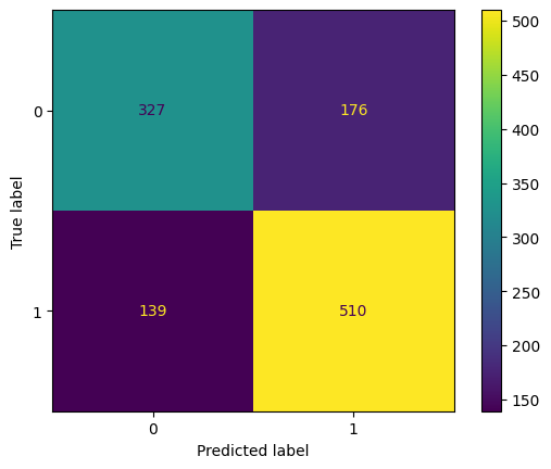
Let first look at the confusion matrix

cm = confusion_matrix(y_test, y_pred)
cm

array([[327, 176],
       [139, 510]], dtype=int64)

to see a prettier confusion matrix

disp = ConfusionMatrixDisplay(confusion_matrix=cm)
disp.plot()

<sklearn.metrics._plot.confusion_matrix.ConfusionMatrixDisplay at 0x29162a1d308>

Now, let’s look at the other metrics

print('{:<10}  {:<15}'.format('Accuracy:', accuracy_score(y_test, y_pred)))
print('{:<10}  {:<15}'.format('Precision:', precision_score(y_test, y_pred)))
print('{:<10}  {:<15}'.format('Recall:', recall_score(y_test, y_pred)))
print('{:<10}  {:<15}'.format('F1:', f1_score(y_test, y_pred)))

Accuracy:   0.7265625      
Precision:  0.7434402332361516
Recall:     0.785824345146379
F1:         0.7640449438202247

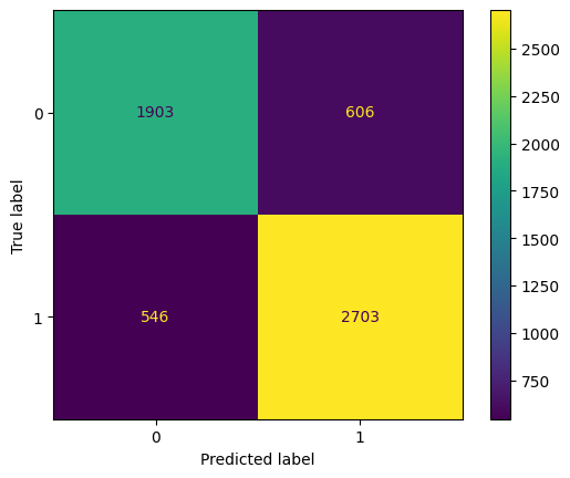
Comparison to VEGA model

What do you think about the metrics? Is the kNN model performing good or bad? Let’s compare it to the predictions of a kNN model trained on this same dataset and published as part of the VEGA platform. In the VEGA model, they have choosen k=4 with a similarity threshold of 0.7 (according to an internal similarity metric) Why is such threshold important?

Also, the developers of the VEGA kNN model used the leave-one-out approach to assess the performace of their model. Why is this approach specially suitable when using the kNN algorithm?

VEGA model

y_clean = df_clean['Experimental value'].astype(int)
y_vega_clean = df_clean['Predicted value'].astype(int)

cm = confusion_matrix(y_clean, y_vega_clean)
disp = ConfusionMatrixDisplay(confusion_matrix=cm)
disp.plot()
print('{:<10}  {:<15}'.format('Accuracy:', accuracy_score(y_clean, y_vega_clean)))
print('{:<10}  {:<15}'.format('Precision:', precision_score(y_clean, y_vega_clean)))
print('{:<10}  {:<15}'.format('Recall:', recall_score(y_clean, y_vega_clean)))
print('{:<10}  {:<15}'.format('F1:', f1_score(y_clean, y_vega_clean)))

Accuracy:   0.7999305314345259
Precision:  0.8168631006346329
Recall:     0.8319482917820868
F1:         0.8243366880146386

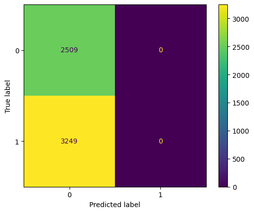
Exercise - leave-one-out cross-validation ❗❗

• Can you now assess our previous kNN model configuration using the leave-one-out approach on the cleaned dataset?

from sklearn.model_selection import LeaveOneOut

X_clean = df_clean.drop(['Unnamed: 0', 'Id','CAS','SMILES','Status','Experimental value','Predicted value'],axis=1)

loo = LeaveOneOut()
print('Number of folds: ', loo.get_n_splits(X_clean))

Number of folds:  5758

y_pred_loo_our_model = np.zeros(y_clean.shape[0])
for i, (train_index, test_index) in enumerate(loo.split(X_clean)):
  # Get training data for the current fold
  X_train_loo = X_clean.iloc[train_index]
  y_train_loo = y_clean.iloc[train_index]

  # Get test data for the current fold
  X_test_loo = X_clean.iloc[test_index]

  # Train kNN
  # Your code here

  # Get prediction on the test molecule
  # Your code here

  # Store the prediction in `y_pred_loo_our_model`
  # Your code here

cm = confusion_matrix(y_clean, y_pred_loo_our_model)
disp = ConfusionMatrixDisplay(confusion_matrix=cm)
disp.plot()
print('{:<10}  {:<15}'.format('Accuracy:', accuracy_score(y_clean, y_pred_loo_our_model)))
print('{:<10}  {:<15}'.format('Precision:', precision_score(y_clean, y_pred_loo_our_model)))
print('{:<10}  {:<15}'.format('Recall:', recall_score(y_clean, y_pred_loo_our_model)))
print('{:<10}  {:<15}'.format('F1:', f1_score(y_clean, y_pred_loo_our_model)))

Accuracy:   0.4357415769364363
Precision:  0.0            
Recall:     0.0            
F1:         0.0            

C:\Users\DELL\Anaconda3\envs\ML4ChemEng\lib\site-packages\sklearn\metrics\_classification.py:1318: UndefinedMetricWarning: Precision is ill-defined and being set to 0.0 due to no predicted samples. Use `zero_division` parameter to control this behavior.
  _warn_prf(average, modifier, msg_start, len(result))

Finding the best k in kNN 🔎

What about the parameter k? How do we find the best k for our model? Why the VEGA model developers used k=4? Let’s try to answer this…

k is a hyperparameter of the model and should be chosen using a validation set.

Important

Remember to reserve your test set exclusively for assesing your model! Never use it for training or hyperparameter tuning!

import numpy as np
from tqdm.notebook import tqdm

num_ks = np.arange(1, 100, 2).astype(int)

X_train_hyp, X_valid, y_train_hyp, y_valid = train_test_split(X_train, y_train, test_size=0.1, random_state=0)

train_accuracy = []
valid_accuracy = []

for i in tqdm(range(len(num_ks))):
  knn = KNeighborsClassifier(n_neighbors=num_ks[i])
  knn.fit(X_train_hyp, y_train_hyp)

  pred_train = knn.predict(X_train_hyp)
  pred_valid  = knn.predict(X_valid)

  train_accuracy.append(1-accuracy_score(y_train_hyp, pred_train))
  valid_accuracy.append(1-accuracy_score(y_valid, pred_valid))

plt.figure(figsize=(10,6))
plt.plot(num_ks, train_accuracy, 'bs--', label='Train')
plt.plot(num_ks, valid_accuracy, 'rx--', label='Validation')
plt.xlabel('k')
plt.ylabel('Misclasification rate')
plt.legend()
plt.show()

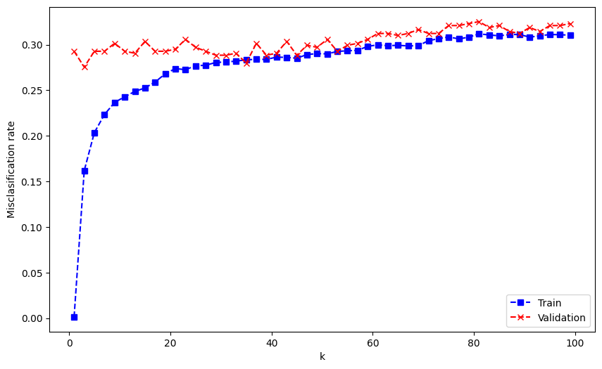
This graph is pretty similar to the one that we saw on slide 9 of Lecture 2. Here, we can see the expected general trend of the performance curves.

Which k do you think is the best?

Cross-validation

Problem: if validation set is small and noisy, it might be misleading Idea: Increase the size of the validation set Problem: This would reduce the size of the training set

Then, let’s use all data for training and validation using k-fold cross-validation!

from sklearn.model_selection import cross_validate

num_ks = np.arange(1, 50, 1).astype(int)

train_misclassification = []
valid_misclassification = []
for i in tqdm(range(len(num_ks))):
  knn = KNeighborsClassifier(n_neighbors=num_ks[i])
  cv_dict = cross_validate(knn, X_train, y_train, cv=10, 
                                 scoring='accuracy', return_train_score=True)
  
  k_fold_train_scored = cv_dict['train_score']
  k_fold_valid_scored = cv_dict['test_score']
  
  train_misclassification.append(1-k_fold_train_scored.mean())
  valid_misclassification.append(1-k_fold_valid_scored.mean())
  

plt.figure(figsize=(10,6))
plt.plot(num_ks, train_misclassification, 'bs--', label='Train')
plt.plot(num_ks, valid_misclassification, 'rx--', label='Validation')
plt.xlabel('k')
plt.ylabel('Misclasification rate')
plt.legend()
plt.show()

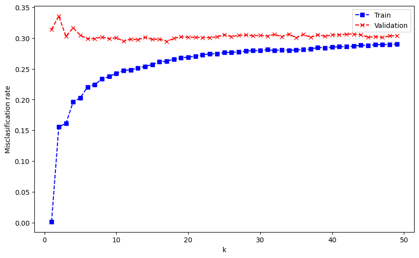
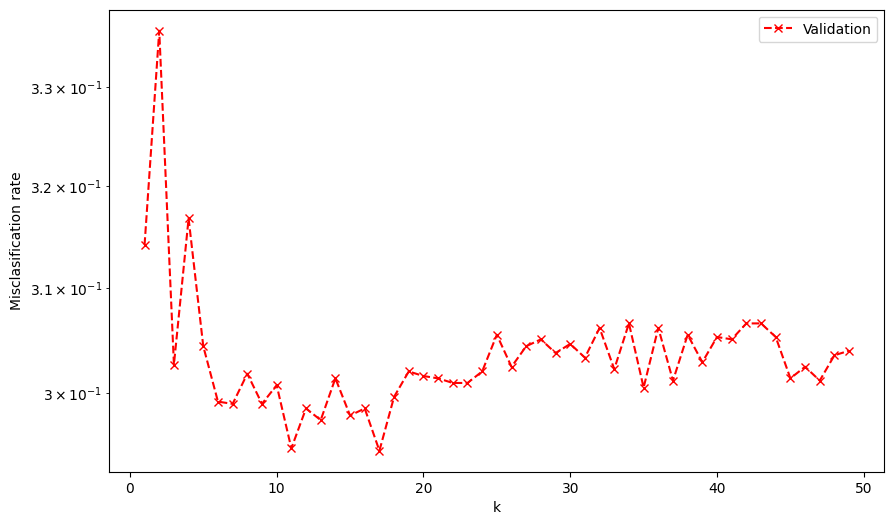
print('k with minimum validation misclassification: ', num_ks[np.argmin(valid_misclassification)])

k with minimum validation misclassification:  17

plt.figure(figsize=(10,6))
plt.plot(num_ks, valid_misclassification, 'rx--', label='Validation')
plt.yscale('log')
plt.xlabel('k')
plt.ylabel('Misclasification rate')
plt.legend()
plt.show()

You can now go back to your implementation of leave-one-out and train your kNN model using the best k that you found. How does it perform compared to the VEGA kNN? Do you got a better model? Why?

Challenge - kNN QSPR for predicting BCF 🥇

Develop a kNN model for regression to predict the bioconcentration factor (BCF).

if 'google.colab' in str(get_ipython()):
  df_bcf = pd.read_csv("https://raw.githubusercontent.com/edgarsmdn/MLCE_book/main/references/BCF_training.csv")
else:
  df_bcf = pd.read_csv("references/BCF_training.csv")

# Your code here

References

HMS+09

Katja Hansen, Sebastian Mika, Timon Schroeter, Andreas Sutter, Antonius Ter Laak, Thomas Steger-Hartmann, Nikolaus Heinrich, and Klaus-Robert Muller. Benchmark data set for in silico prediction of ames mutagenicity. Journal of chemical information and modeling, 49(9):2077–2081, 2009.

Mur22

Kevin P Murphy. Probabilistic machine learning: an introduction. MIT press, 2022.

SXG+03

Min Shen, Yunde Xiao, Alexander Golbraikh, Vijay K Gombar, and Alexander Tropsha. Development and validation of k-nearest-neighbor qspr models of metabolic stability of drug candidates. Journal of medicinal chemistry, 46(14):3013–3020, 2003.

YJQ+19

Shuai Yuan, Zeren Jiao, Noor Quddus, Joseph Sang-II Kwon, and Chad V Mashuga. Developing quantitative structure–property relationship models to predict the upper flammability limit using machine learning. Industrial & Engineering Chemistry Research, 58(8):3531–3537, 2019.