1. Introduction to Python 🐍

This Notebook was originally prepared by Mathieu Blondel and few modifications have been made by us.

Goals of this exercise 🌟

• We will learn about the programming language Python as well as NumPy and Matplotlib, two fundamental tools for data science and machine learning in Python.

What are Jupyter Notebooks and Google Colab? 🤔

Notebooks are a great way to mix executable code with rich contents (HTML, images, equations written in LaTeX). Google Colab allows to run notebooks on the cloud for free without any prior installation, while leveraging the power of GPUs.

This document that you are reading is not a static web page, but an interactive environment called a notebook, that lets you write and execute code. Notebooks consist of so-called code cells, blocks of one or more Python instructions. For example, here is a code cell that stores the result of a computation (the number of seconds in a day) in a variable and prints its value:

seconds_in_a_day = 24 * 60 * 60
seconds_in_a_day

86400

Click on the “play” button to execute the cell. You should be able to see the result. Alternatively, you can also execute the cell by pressing Ctrl + Enter if you are on Windows/Linux or Command + Enter if you are on a Mac.

Variables that you defined in one cell can later be used in other cells:

seconds_in_a_week = 7 * seconds_in_a_day
seconds_in_a_week

604800

Note that the order of execution is important. For instance, if we do not run the cell storing seconds_in_a_day beforehand, the above cell will raise an error, as it depends on this variable. To make sure that you run all the cells in the correct order, you can also click on Runtime in the top-level menu, then Run all.

Exercise - code cells ❗❗

Add a code cell below this cell:

1. Click on this cell

2. Click on + Code

3. In the new cell, compute the number of seconds in a year by reusing the variable seconds_in_a_day. Run the new cell.

Python 🐍

Python is one of the most popular programming languages for machine learning, both in academia and in industry. As such, it is essential to learn this language for anyone interested in machine learning. In this section, we will review Python basics.

Arithmetic operations

Python supports the usual arithmetic operators: + (addition), * (multiplication), / (division), ** (power), // (integer division).

Lists

Lists are a container type for ordered sequences of elements. Lists can be initialized empty

my_list = []

or with some initial elements

my_list = [1, 2, 3]

Lists have a dynamic size and elements can be added (appended) to them

my_list.append(4)
my_list

[1, 2, 3, 4]

We can access individual elements of a list (indexing starts from 0)

my_list[2]

3

We can access “slices” of a list using my_list[i:j] where i is the start of the slice (again, indexing starts from 0) and j the end of the slice. For instance:

my_list[1:3]

[2, 3]

Omitting the second index means that the slice shoud run until the end of the list

my_list[1:]

[2, 3, 4]

We can check if an element is in the list using in

5 in my_list

False

The length of a list can be obtained using the len function

len(my_list)

4

Strings

Strings are used to store text. They can be defined using either single quotes or double quotes

string1 = "some text"
string2 = 'some other text'

Strings behave similarly to lists. As such we can access individual elements in exactly the same way

string1[3]

'e'

and similarly for slices

string1[5:]

'text'

String concatenation is performed using the + operator

string1 + " " + string2

'some text some other text'

Conditionals

As their name indicates, conditionals are a way to execute code depending on whether a condition is True or False. As in other languages, Python supports if and else but else if is contracted into elif, as the example below demonstrates.

my_variable = 5
if my_variable < 0:
  print("negative")
elif my_variable == 0:
  print("null")
else: # my_variable > 0
  print("positive")

positive

Here < and > are the strict less and greater than operators, while == is the equality operator (not to be confused with =, the variable assignment operator). The operators <= and >= can be used for less (resp. greater) than or equal comparisons.

Contrary to other languages, blocks of code are delimited using indentation. Here, we use 2-space indentation but many programmers also use 4-space indentation. Any one is fine as long as you are consistent throughout your code.

Loops

Loops are a way to execute a block of code multiple times. There are two main types of loops: while loops and for loops.

While loop

i = 0
while i < len(my_list):
  print(my_list[i])
  i += 1 # equivalent to i = i + 1

1
2
3
4

For loop

for i in range(len(my_list)):
  print(my_list[i])

1
2
3
4

If the goal is simply to iterate over a list, we can do so directly as follows

for element in my_list:
  print(element)

1
2
3
4

Functions

To improve code readability, it is common to separate the code into different blocks, responsible for performing precise actions: functions! 😃 A function takes some inputs and process them to return some outputs.

def square(x):
  return x ** 2

def multiply(a, b):
  return a * b

# Functions can be composed.
square(multiply(3, 2))

36

To improve code readability, it is sometimes useful to explicitly name the arguments

square(multiply(a=3, b=2))

36

Exercise - conditionals, loops and function ❗❗

Exercise 1. Using a conditional, write the relu function defined as follows

\(\text{relu}(x) = \left\{ \begin{array}{rl} x, & \text{if } x \ge 0 \\ 0, & \text{otherwise }. \end{array}\right.\)

def relu(x):
  # Write your function here
  return

relu(-3)

Exercise 2. Using a foor loop, write a function that computes the Euclidean norm of a vector, represented as a list.

def euclidean_norm(vector):
  # Write your function here
  return

my_vector = [0.5, -1.2, 3.3, 4.5]
# The result should be roughly 5.729746940310715
euclidean_norm(my_vector)

Exercise 3. Using a for loop and a conditional, write a function that returns the maximum value in a vector.

def vector_maximum(vector):
  # Write your function here
  return

Bonus exercise. if time permits, write a function that sorts a list in ascending order (from smaller to bigger) using the bubble sort algorithm.

def bubble_sort(my_list):
  # Write your function here
  return

my_list = [1, -3, 3, 2]
# Should return [-3, 1, 2, 3]
bubble_sort(my_list)

Going further 💯

Clearly, it is impossible to cover all the language features in this short introduction. To go further, we recommend the following resources:

• Python for for computations in science and engineering booklets.

• List of Python tutorials

• Four-hour course on Youtube

NumPy 💻

NumPy is a popular library for storing arrays of numbers and performing computations on them. Not only this enables to write often more succint code, this also makes the code faster, since most NumPy routines are implemented in C for speed.

To use NumPy in your program, you need to import it as follows

import numpy as np

Array creation

NumPy arrays can be created from Python lists

my_array = np.array([1, 2, 3])
my_array

array([1, 2, 3])

NumPy supports array of arbitrary dimension. For example, we can create two-dimensional arrays (e.g. to store a matrix) as follows

my_2d_array = np.array([[1, 2, 3], [4, 5, 6]])
my_2d_array

array([[1, 2, 3],
       [4, 5, 6]])

We can access individual elements of a 2d-array using two indices

my_2d_array[1, 2]

6

We can also access rows

my_2d_array[1]

array([4, 5, 6])

and columns

my_2d_array[:, 2]

array([3, 6])

Arrays have a shape attribute

print(my_array.shape)
print(my_2d_array.shape)

(3,)
(2, 3)

Contrary to Python lists, NumPy arrays must have a type and all elements of the array must have the same type.

my_array.dtype

dtype('int32')

The main types are int32 (32-bit integers), int64 (64-bit integers), float32 (32-bit real values) and float64 (64-bit real values).

The dtype can be specified when creating the array

my_array = np.array([1, 2, 3], dtype=np.float64)
my_array.dtype

dtype('float64')

We can create arrays of all zeros using

zero_array = np.zeros((2, 3))
zero_array

array([[0., 0., 0.],
       [0., 0., 0.]])

and similarly for all ones using ones instead of zeros.

We can create a range of values using

np.arange(5)

array([0, 1, 2, 3, 4])

or specifying the starting point

np.arange(3, 5)

array([3, 4])

Another useful routine is linspace for creating linearly spaced values in an interval. For instance, to create 10 values in [0, 1], we can use

np.linspace(0, 1, 10)

array([0.        , 0.11111111, 0.22222222, 0.33333333, 0.44444444,
       0.55555556, 0.66666667, 0.77777778, 0.88888889, 1.        ])

Another important operation is reshape, for changing the shape of an array

my_array = np.array([1, 2, 3, 4, 5, 6])
my_array.reshape(3, 2)

array([[1, 2],
       [3, 4],
       [5, 6]])

Play with these operations and make sure you understand them well.

Basic operations

In NumPy, we express computations directly over arrays. This makes the code much more succint.

Arithmetic operations can be performed directly over arrays. For instance, assuming two arrays have a compatible shape, we can add them as follows

array_a = np.array([1, 2, 3])
array_b = np.array([4, 5, 6])
array_a + array_b

array([5, 7, 9])

Compare this with the equivalent computation using a for loop

array_out = np.zeros_like(array_a)
for i in range(len(array_a)):
  array_out[i] = array_a[i] + array_b[i]
array_out

array([5, 7, 9])

Not only this code is more verbose, it will also run much more slowly.

In NumPy, functions that operates on arrays in an element-wise fashion are called universal functions. For instance, this is the case of np.sin

np.sin(array_a)

array([0.84147098, 0.90929743, 0.14112001])

Vector inner product can be performed using np.dot

np.dot(array_a, array_b)

32

When the two arguments to np.dot are both 2d arrays, np.dot becomes matrix multiplication

array_A = np.random.rand(5, 3)
array_B = np.random.randn(3, 4)
np.dot(array_A, array_B)

array([[ 0.04331007, -0.12732298, -0.37327668,  0.05407328],
       [ 1.34376525, -0.34107647, -2.8919084 ,  0.51273673],
       [-0.1888115 ,  0.05371448, -1.61399028, -0.38581737],
       [ 0.37507065,  0.00382352, -2.5611779 , -0.19433127],
       [ 0.7794883 ,  0.26689005, -3.1714363 , -0.2531818 ]])

Matrix transpose can be done using .transpose() or .T for short

array_A.T

array([[0.09265561, 0.20253672, 0.7147417 , 0.71531712, 0.73346626],
       [0.25471784, 0.43083481, 0.84483282, 0.81372203, 0.46602803],
       [0.05729811, 0.92323932, 0.06229396, 0.42365698, 0.67390611]])

Slicing and masking

Like Python lists, NumPy arrays support slicing

np.arange(10)[5:]

array([5, 6, 7, 8, 9])

We can also select only certain elements from the array

x = np.arange(10)
mask = x >= 5
x[mask]

array([5, 6, 7, 8, 9])

Exercise - arrays and linear algebra ❗❗

Exercise 1. Create a 3d array of shape (2, 2, 2), containing 8 values. Access individual elements and slices.

# Your code here

Exercise 2. Rewrite the relu function (see Python section) using np.maximum. Check that it works on both a single value and on an array of values.

def relu_numpy(x):
  return

relu_numpy(np.array([1, -3, 2.5]))

Exercise 3. Rewrite the Euclidean norm of a vector (1d array) using NumPy (without for loop)

def euclidean_norm_numpy(x):
  return

my_vector = np.array([0.5, -1.2, 3.3, 4.5])
euclidean_norm_numpy(my_vector)

Exercise 4. Write a function that computes the Euclidean norms of a matrix (2d array) in a row-wise fashion. Hint: use the axis argument of np.sum.

def euclidean_norm_2d(X):
  return

my_matrix = np.array([[0.5, -1.2, 4.5],
                      [-3.2, 1.9, 2.7]])
# Should return an array of size 2.
euclidean_norm_2d(my_matrix)

Exercise 5. Compute the mean value of the features in the iris dataset. Hint: use the axis argument on np.mean.

from sklearn.datasets import load_iris
X, y = load_iris(return_X_y=True)

# Result should be an array of size 4.

Going further 💯

• NumPy reference

• SciPy lectures

• One-hour tutorial on Youtube

Matplotlib 📈

Basic plots

Matplotlib is a plotting library for Python.

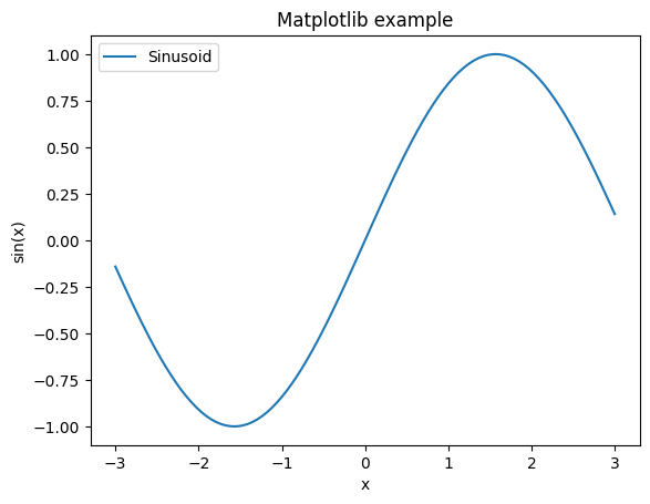
We start with a rudimentary plotting example.

from matplotlib import pyplot as plt

x_values = np.linspace(-3, 3, 100)

plt.figure()
plt.plot(x_values, np.sin(x_values), label="Sinusoid")
plt.xlabel("x")
plt.ylabel("sin(x)")
plt.title("Matplotlib example")
plt.legend(loc="upper left")
plt.show()

We continue with a rudimentary scatter plot example. This example displays samples from the iris dataset using the first two features. Colors indicate class membership (there are 3 classes).

from sklearn.datasets import load_iris
X, y = load_iris(return_X_y=True)

X_class0 = X[y == 0]
X_class1 = X[y == 1]
X_class2 = X[y == 2]

plt.figure()
plt.scatter(X_class0[:, 0], X_class0[:, 1], label="Class 0", color="C0")
plt.scatter(X_class1[:, 0], X_class1[:, 1], label="Class 1", color="C1")
plt.scatter(X_class2[:, 0], X_class2[:, 1], label="Class 2", color="C2")
plt.show()

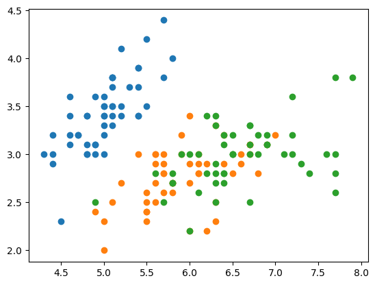
We see that samples belonging to class 0 can be linearly separated from the rest using only the first two features.

Exercise - plots ❗❗

Exercise 1. Plot the relu and the softplus functions on the same graph.

# Your code here

What is the main difference between the two functions?

Exercise 2. Repeat the same scatter plot but using the digits dataset instead.

from sklearn.datasets import load_digits
X, y = load_digits(return_X_y=True)

Are pixel values good features for classifying samples?

Going further 💯

• Official tutorial

• Tutorial on Youtube